The link to the ArcGIS Pro toolbox and QGIS plugin to create and view the camelplots for the ICE-D dataset in ArcGIS Pro and QGIS can be found at: https://github.com/yingkui2003/ICE-DTools.

The ArcGIS Pro toolbox can be directly used in ArcGIS Pro after adding a folder connection of the ArcGIS Pro toolbox folder to the ArcGIS Pro project. This toolbox includes three tools:

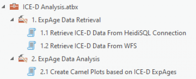
The “Retrieve ICE-D Data From HeidiSQL Connection” tool is used to retrieve exposure ages (ICE-D Alpine) based on specified latitude and longitude ranges. The user also needs to select a scaling model for the ages (St, Lm, or LSDn).

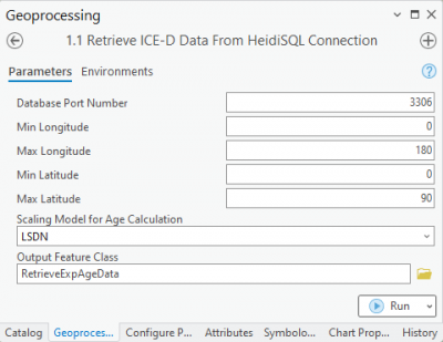
Note that this tool is limited to the computer that has the HeidiSQL and ICE-D database installed. The user also needs to keep the ICE-D database open to run this tool. In addition, the pymysql, shapely, and fiona libraries are also needed to be installed in the ArcGIS Pro python version. To do that, open the “Python Command Prompt” under the ArcGIS Pro program folder by clicking the Microsoft Window icon on the left-bottom bar of the computer and find the ArcGIS or ArcGIS Pro app folder. Then, run the following commands:

pip install pymysql
pip install shapely
pip install fiona

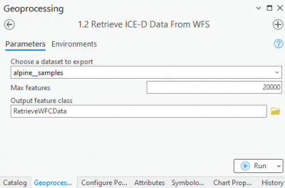
The ICE-D dataset can be imported into ArcGIS Pro as a WFS layer. However, ArcGIS Pro uses a limit of 3000 for the ICE-D dataset. To retrieve more exposure ages, a new tool, “Retrieve ICE-D Data From WFS”, is developed. The users can select a dataset from ICE-D and provide a maximum number of features to retrieve the exposure ages as a feature class in ArcGIS Pro.

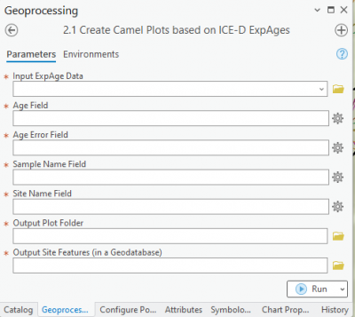
The “Create Camel Plots based on ICE-D ExpAges” tool is developed to create the camelplot for each site based on multiple exposure ages. All camelplots are saved into a folder and a site feature class is created to save the summary info of the exposure ages, such as mean, std, variances, skewness, and chi-square values. Each camelplot is also associated with its corresponding site so that the plot can be viewed interactively in ArcGIS Pro. The following is a screenshot of the interface of this tool in ArcGIS Pro.

How to install and use the ICE-D Analysis plugin in QGIS

1) Find the “iced_camelplots” folder after unzipping the downloaded file from GitHub and check if there are a set of folders and files (similar to the following screenshot) within the folder:

2) Open QGIS and under the “Setting” menu, choose User profile → Open Active Profile Folder. See the following screenshot.

This will open the active profile folder. Then, copy the “iced_camelplots” folder to the “python→plugins” folder in the active profile folder. If there is no the “plugins” folder, create one.

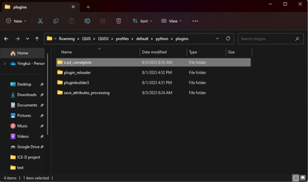
3) Close and reopen QGIS. Under the “Plugin” menu, Click “Manage and Install Plugins…”.

On the left panel of the Plugins window, Click “Installed” and You should find the “ICE-D Camelplots” plugin (the following screenshot). Chick it and close the window.

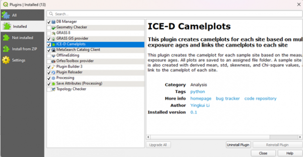
Note that this plugin is in development mode. More functions will be added in the future. After the plugin is finalized, it can be published directly in QGIS, so that no copy/paste folder is needed in the future.

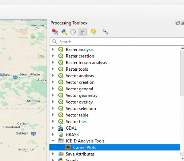
4) You should be able to see the plugin in three locations: the Plugin menu, the toolbar, and the processing toolbox.

You can run the “Camel Plots” tool from one of these three locations.

How to use the “Camel Plots” tool and view the camelplots in QGIS

The following screenshot shows the interface of the “Camel Plots” tool after running it.

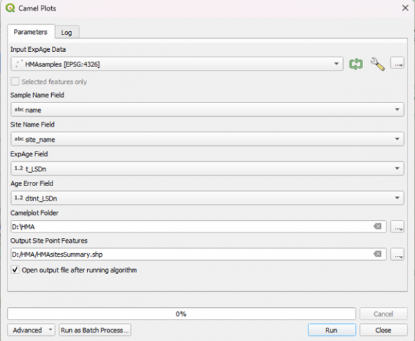
You need to specify the ExpAge data (a subset layer of the WFS feature of the ICE-D database), then select the Sample Name Field (name), Site Name Field (site_name), ExpAge Field (t_LSDn or t_St), and Age Error Field (t_dint_LSDn or t_dint_St). You also need to choose a folder to save the camelplot for each site and an Output Site Point Feature as a shapefile or other GIS format. After that, click Run to run the tool.

The progress bar will show the progress of the calculation. After finishing, a site point layer will be added to the map to show the summary (#samples, mean, std, variance, skewness, and Chi-square) of each site and the link to the camelplot images. The following is a screenshot of the attribute table of the created site layer.

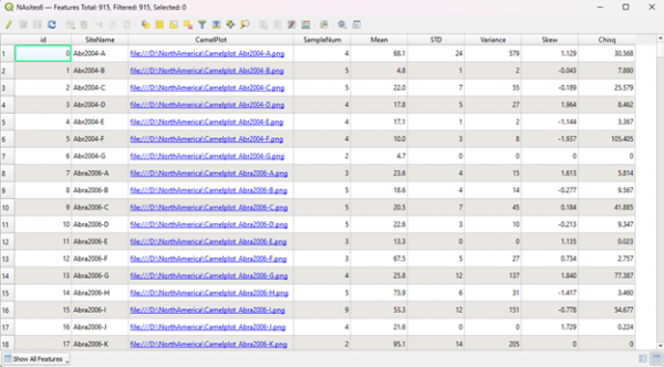
You can “Ctrl + Click” the image path to view the camelplot for each site. You can also view the camelplot in QGIS as HTML map tips. To enable this function, right-click the created site layer and choose “Properties”. In the Layer Properties Dialog, click “Display” on the left panel.

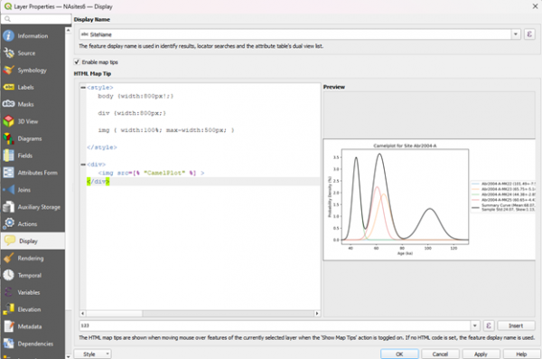
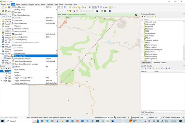
Make sure to check “Enable Map tips” (QGIS 3.32). If using the old version of QGIS, you need to Click the “View” menu and click “Show Map Tips” to enable this function (see the following screenshot).

In the Layer Properties Dialog, add the following part to the box under “HTML Map Tip”:

<style>
   body {width:800px!;}
   div {width:800px;} 
   img { width:100%; max-width:500px; }
</style>
<div>
   <img src=[% "CamelPlot" %] > 
</div> 

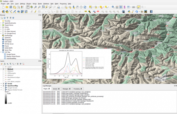
Click OK. This will show the camelplot as a map tip when the cursor is close to each site (the site layer needs to be selected). The following screenshot is an example.