A WFS service provided by a Geoserver installation allows display and analysis of ICE-D exposure age data within desktop GIS software such as ArcGIS and QGIS. This means that whenever there are updates to the data in ICE-D (e.g., users add new data to ICE-D), the WFS also gets updated and so as long as you have an internet connection, you will be viewing the latest and most up-to-date account of samples in ICE-D in your own personal desktop application!

Connecting in QGIS:

In the QGIS “browser” panel (can be shown on the page by navigating to view → panel → and selecting “browser”) one of the options for layers to add to any map is the “WFS / OGC API - features” option. Right click that option and select “New Connection…”

The new connection window should look like this:

Name the connection whatever you like, I named mine iced.

In the URL line, add in the following URL:

https://geoserver.ice-d.org/geoserver/wfs?version=2.0.0

This link establishes a connection between your desktop GIS application and all of the ICE-D data stored as a Web Feature Service (WFS) hosted online by Geoserver. Before selecting OK, be sure to check the box stating “Invert axis orientation”. Otherwise QGIS will think latitude values are longitude values and vice versa and all of your sample locations will be rotated 90 degrees. After checking the box select OK.

This entire process can also be done from the top drop down menus. Select Layer → Data source manager and the following page should open:

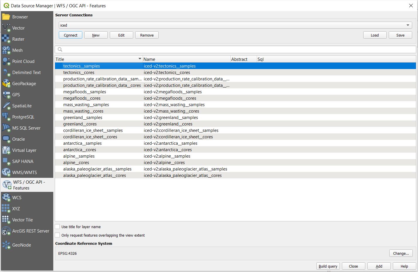
In the screenshot I am showing what the page should look like if the connection is successful (note that the box titled Only request features overlapping the view extent is UNCHECKED). Here, you would select the “New” option and the New Connection window will appear as it did through the previous route.

Once you properly set up the new connection and select OK, there should be a new drop down menu below the “WFS / OGC API Features” option with whatever name you gave to the ICE-D WFS connection you just made. under the connection, there should be a list of layers. Also, when you select the “Connect” option in the data source manager window, you should see the same list of layers. As discussed in more detail below, each application has its own set of two layers; one for surface samples that belong to the application and one for core samples that belong to the application.

Each application in ICE-D (e.g., ICE-D Greenland, ICE-D Alpine, ICE-D Tectonics, etc.) has its own set of two layers:

1) All the surface samples associated with an application.

2) All the core samples associated with an application.

For example, loading up every sample that belongs to the Greenland Database will look something like this:

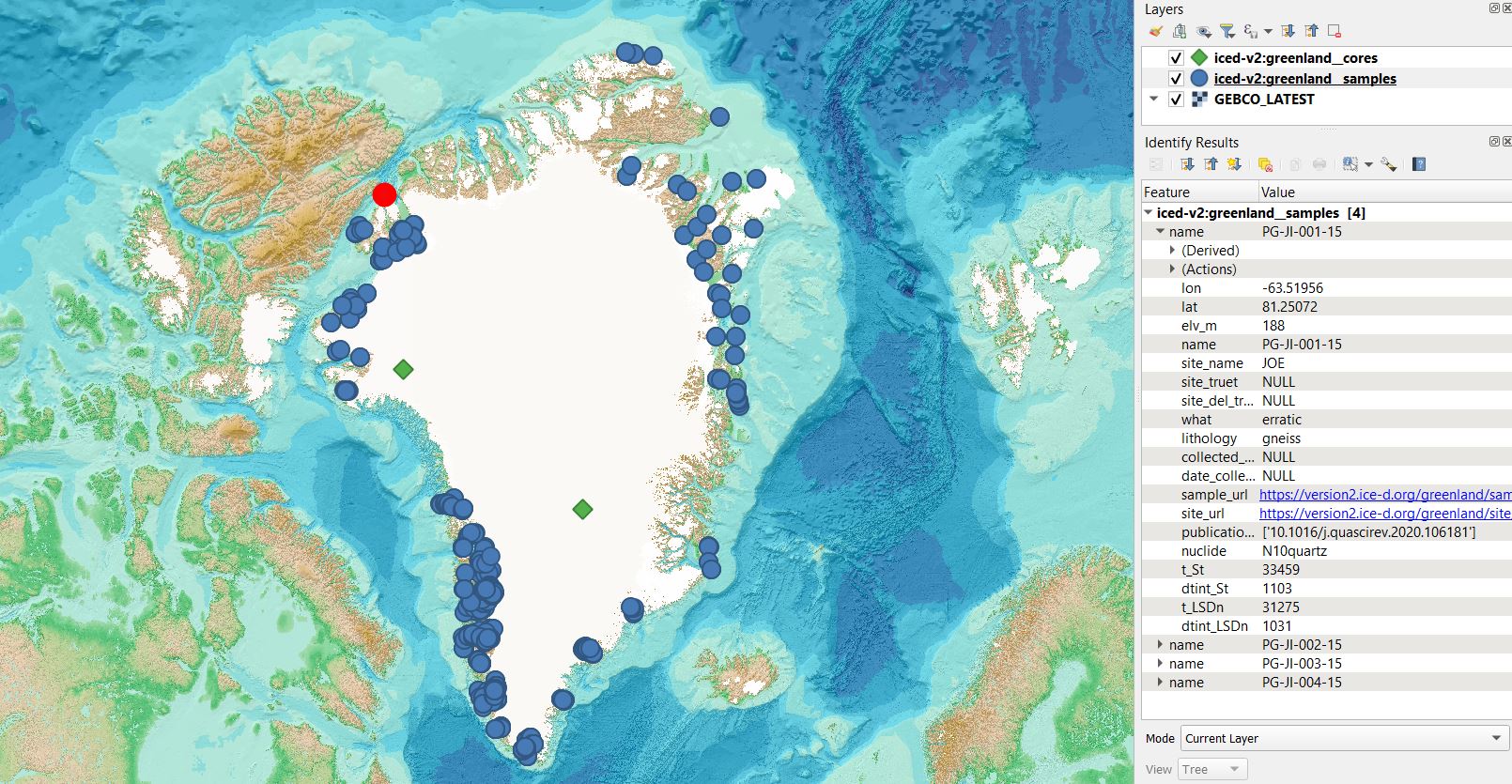
Green triangles are core data and blue dots are surface sample data. See description below of attribute data.

In the image above, I selected some random surface samples related to the Greenland Ice Sheet in northwest Greenland as an example (the red highlighted dots on the map). Each entry (sample) has a set amount of attribute data that comes from ICE-D. The image shows the complete list, and users are encouraged to explore on their own, but attribute data includes lat lon and sample elevation values, among other attributes useful for querying. Currently, each sample has reported calculated ages based on the default production rate (Borchers et al., 2016) and the scaling scheme from Stone (2000) (St) and from Lifton et al. (2014) (LSDn). Attribute data also includes links to sample and site pages and a list of DOI's to publications associated with each sample.

A major advantage of viewing samples in your own personal desktop application is that you have access to all of the samples in the database and their metadata, and you can select samples based on geographic locations with ease. However, GIS applications also have querying tools that allow users to select samples based on their attributes in essentially the same exact way a user might query an sql database to extract the exact data they want. Please find an example of using QGIS to query data from ICE-D in the ICE-D tutorials, visualization and analysis applications page